Clustering Sparse Codes

Sparse codes are not just smaller — they are organized. Each row is a short list of signed features, and rows that share features tend to be semantically related. compresso.clustering turns that structure into an interpretable hierarchy of clusters.

This page is a hands-on walkthrough on a real dataset: the Goodbooks-10k collection of 10,000 books. We embed each book’s text, compress the embeddings into sparse codes, and cluster the codes into book “themes” — then label those themes with Goodreads shelf tags. All figures on this page come from docs/gen_figures.py.

The idea

A standard clustering algorithm (k-means, agglomerative) works on dense vectors and asks “which points are close?”. Compresso’s clustering instead works on sparse activation patterns and asks “which entities switch on the same features?”. Because a top-k SAE feature usually corresponds to one concept, a group of entities sharing a feature is a ready-made, explainable cluster — no distance threshold to tune for the first cut, and the cluster comes with the feature(s) that define it.

Step 1 — from text to sparse codes

We start from dense text embeddings (any sentence encoder works) and compress them with a top-k SAE exactly as in Getting Started:

import numpy as np
from sentence_transformers import SentenceTransformer
from compresso import TopKSAEConfig, TopKSAETrainer

# text = ["<title>. by <authors>. <description>", ...] for 10k books
encoder = SentenceTransformer("sentence-transformers/all-MiniLM-L6-v2")
emb = encoder.encode(text, normalize_embeddings=True).astype("float32")  # (10000, 384)

srp = TopKSAETrainer(
    TopKSAEConfig(hidden_dim=1024, k=32, epochs=80, decay=True, seed=0)
).fit_transform(emb)                                                       # (10000, 1024), k=32

(If you persisted codes earlier, srp = load_srp_tensor(...) — see Input and Output.)

Step 2 — build a clustering pipeline

A ClusteringPipeline is an ordered list of steps applied to the SRPTensor. Each step is a small, named transform, so the recipe reads top-to-bottom:

import compresso.clustering as cc

clusters = cc.ClusteringPipeline([
    cc.TopMSignedClustering(top_m=2, min_cluster_size=10),     # 1. seed clusters
    cc.EntityContainmentLink(threshold=0.9),                   # 2. find nested clusters
    cc.MaterializeLinkMerges(parent_scope="active"),           # 3. merge along those links
    cc.PruneRedundantRoots(),                                  # 4. drop subsumed clusters
    cc.AssignTags(entity_tag_matrix=tags, tag_names=tag_names, # 5. label with shelf tags
                  method="tfidf", top_k=8),
    cc.SizeFilter(min_cluster_size=15),                        # 6. keep sizeable clusters
]).fit(srp)

What each stage does:

1. Clustering (TopMSignedClustering) seeds clusters from activation patterns: entities are grouped by their top-m signed features, so a feature firing positively and negatively yields two distinct groups. Other seed strategies are available (DominantSignedClustering, ComboSignedClustering, SRPSimilarityClustering).

2. Linking (EntityContainmentLink) records when one cluster’s members are (almost) a subset of another’s, without merging yet.

3. Materializing (MaterializeLinkMerges) turns those links into actual parent clusters, building a hierarchy.

4. Pruning (PruneRedundantRoots) deactivates clusters that are fully contained in a larger active one, so the active frontier is clean.

5. Tagging (AssignTags) aggregates an entity-tag matrix over each cluster’s members and stores the top tags, "tfidf" down-weighting globally common tags.

6. Filtering (SizeFilter) keeps only clusters above a size — note this changes the active set; every cluster is still inspectable via clusters.clusters.

fit returns a SparseClusterSet. Filtered and merged-away clusters remain in the graph; the ones that matter are the active frontier, clusters.active_clusters.

Step 3 — the entity-tag matrix (optional labels)

AssignTags is what makes the clusters self-describing. It takes a (n_entities, n_tags) matrix (dense or SciPy sparse) of tag counts/weights and the column names. For Goodbooks we build it from the Goodreads shelf tags (fantasy, self-help, …); any per-entity label source works — genres, categories, keyword flags. Tags are stored on each cluster as ScoredTag objects with name, score, and count.

For LLM- or rule-based free-text labels, LabelClusters runs a user-supplied callback over the clusters; Compresso coordinates the loop but you own the model and prompt.

What you get

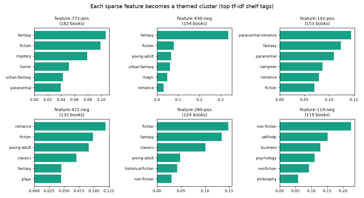
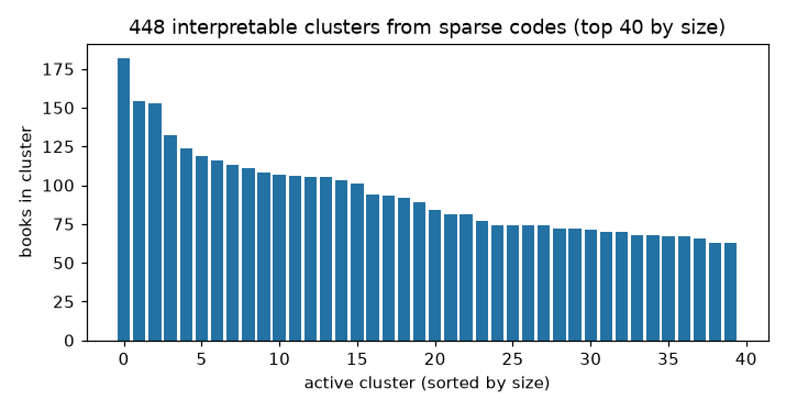
On Goodbooks this yields a few hundred active clusters. Each one corresponds to a sparse feature and lines up with a recognizable book theme — from contemporary romance to self-help to religion:

feature:471:neg  n=132  tags=[romance, fiction, young-adult, classics]
                 e.g. Twilight; Romeo and Juliet; The Notebook
feature:119:neg  n=119  tags=[non-fiction, self-help, business, psychology]
                 e.g. How to Win Friends and Influence People; The Purpose Driven Life
feature:176:neg  n=113  tags=[fiction, romance, young-adult, contemporary]
                 e.g. Me Before You; Never Let Me Go; P.S. I Love You
feature:258:pos  n=108  tags=[christian, non-fiction, religion, fiction]
                 e.g. The Shack; A Prayer for Owen Meany; The God Delusion

The largest themes and their defining shelf tags:

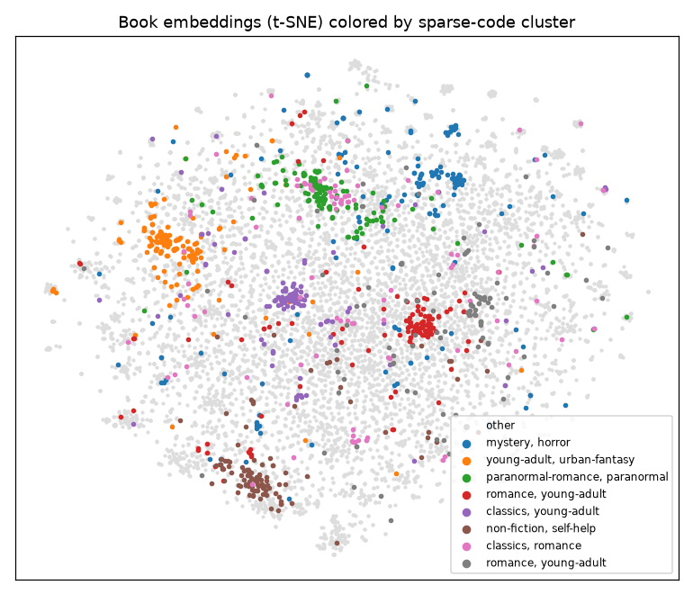
Crucially, these clusters were found from the sparse codes alone. Projecting the original dense embeddings to 2D and coloring by cluster shows the sparse groups land on coherent regions of the embedding space — the compression kept the semantics:

Inspecting clusters

A SparseClusterSet is easy to walk:

for c in sorted(clusters.active_clusters, key=lambda c: -c.entity_count)[:10]:
    tags = ", ".join(f"{t.name}:{t.score:.2f}" for t in c.tags[:5])
    members = titles[c.entity_indices[:5]]          # your own metadata table
    print(c.cluster_id, c.entity_count, "|", tags)
    print("  ", "; ".join(members))

    # the feature(s) that define the cluster:
    print("  centroid features:", c.centroid.indices.tolist())

which prints the largest themes, the books in them, and the sparse feature each one is built on:

feature:772:pos 182 | fantasy:0.11, fiction:0.10, mystery:0.08, horror:0.05, urban-fantasy:0.04
   World War Z: An Oral History of the Zombie War; Pet Sematary; The Graveyard Book; Speaker for the Dead (Ender's Saga, #2); The Walking Dead, Vol. 01
  centroid features: [772]
feature:430:neg 154 | fantasy:0.34, fiction:0.08, young-adult:0.07, urban-fantasy:0.06, magic:0.05
   The Night Circus; Ella Enchanted; The Magician's Nephew (Chronicles of Narnia, #6); The Color of Magic (Discworld, #1); The Velveteen Rabbit
  centroid features: [430]
feature:142:pos 153 | paranormal-romance:0.14, fantasy:0.12, paranormal:0.11, vampires:0.09, romance:0.08
   Dark Places; Sharp Objects; Heart of Darkness; The Subtle Knife (His Dark Materials, #2); Dark Lover (Black Dagger Brotherhood, #1)
  centroid features: [142]

Each cluster is defined by a single sparse feature (centroid features), and its members and shelf tags agree — a self-explaining group, not an opaque cluster id.

Useful members:

• clusters.active_clusters — the current frontier (after pruning/filtering).

• clusters.clusters — every cluster, including merged/filtered nodes.

• clusters.cluster_by_id[cid] — look up one cluster.

• cluster.entity_indices / entity_count — row indices and size.

• cluster.centroid — the defining sparse feature vector (indices/values).

• cluster.tags / cluster.label — assigned tags and optional text label.

• cluster.parent_cluster_ids / child_cluster_ids — hierarchy links.

Saving cluster graphs

Cluster graphs round-trip to disk, so you can compute once and explore later:

from compresso.clustering import save_cluster_graph, load_cluster_graph

save_cluster_graph(clusters, "clusters.json")
clusters = load_cluster_graph("clusters.json")

# or as plain dicts for custom storage:
from compresso.clustering import graph_to_dict, graph_from_dict
payload = graph_to_dict(clusters)

Other building blocks

The pipeline steps are mix-and-match. Besides the seeds and links above, merges include EntityIoUMerge (Jaccard overlap of members), CentroidSimilarityMerge, EntityContainmentMerge, and SemanticSimilarityMerge; AssignUnclusteredToNearestCluster sweeps up leftovers. A lower-level functional API (cc.cluster_srp(...) and cc.run_clustering_pipeline(...)) exists for one-call experiments, but the class-based ClusteringPipeline shown here is the recommended surface.

Note

The clustering API is the most actively developed part of Compresso. The pipeline-and-graph-types surface documented here is the intended entry point; the lower-level builder/merge functions may change.