A First Example: Seeing What an SAE Learns

The quickest way to build intuition for a top-k sparse autoencoder is to train one on images and look at the result, because every learned feature can be drawn as a picture. This example uses MNIST, the classic handwritten-digit images (28×28 grayscale, available through the datasets library), but nothing here is digit-specific: any dense matrix works the same way.

Everything below uses only the high-level public API (TopKSAEConfig, TopKSAETrainer).

Note

This page is illustrative; you do not need to run it to use Compresso. The figures are regenerated by docs/gen_figures.py (see that script for the extra plotting/data dependencies).

Treat each image as a dense vector

We flatten every 28×28 image into a length-784 vector and scale it to [0, 1]. That gives a dense matrix X of shape (n, 784) — exactly the input format the trainer expects.

import numpy as np
from datasets import load_dataset

ds = load_dataset("ylecun/mnist", split="train")
imgs = np.stack([np.asarray(im, dtype=np.float32) for im in ds["image"][:20_000]]) / 255.0
X = imgs.reshape(len(imgs), -1)   # (20000, 784) dense embeddings

Train a top-k SAE

We use a mildly overcomplete code (hidden_dim=196 features) and keep only k=20 of them active per image:

from compresso import TopKSAEConfig, TopKSAETrainer

trainer = TopKSAETrainer(
    TopKSAEConfig(
        hidden_dim=196,
        k=20,
        batch_size=512,
        epochs=60,
        lr=1e-3,
        decay=True,
        seed=0,
    )
).fit(X)

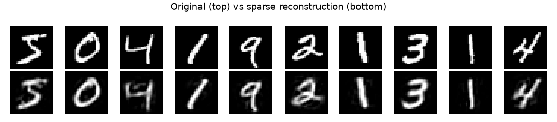
Reconstruction quality climbs quickly. With only 20 active features the reconstructions are recognizably the original digits:

The decoder is a dictionary

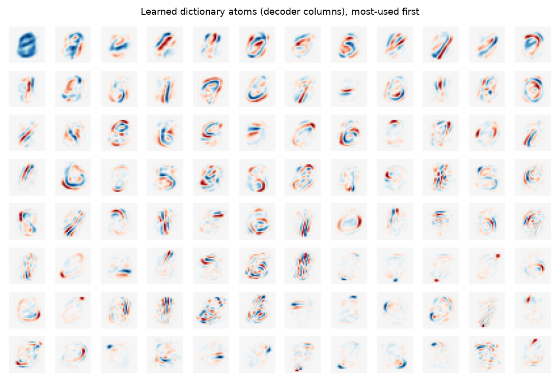
The interesting part is what the model learned. The decoder maps each of the 196 code features back to image space, so every column of the decoder weight is itself a 28×28 image — a dictionary atom. TopKSAE exposes this matrix directly:

W = trainer.sae.get_decoder_weight().detach()   # (784, 196): each column is an atom

Plotted as images (most-used first), the atoms are clearly stroke- and template-like: loops, diagonals, and digit fragments that combine to form glyphs.

A code is a recipe

Because the decoder is linear, the reconstruction of any image is just the weighted sum of its few active atoms. We can read a single image’s sparse code, then watch the picture assemble atom by atom:

code = trainer.encode(X[:1]).numpy()[0]      # (196,), only 20 non-zero
active = np.nonzero(code)[0]                  # which atoms fired
contributions = W.numpy()[:, active] * code[active]   # (784, 20) pieces
reconstruction = contributions.sum(axis=1)   # == trainer.reconstruct(X[:1])

This is the whole idea in one picture: a dense image becomes a short, signed recipe over a shared dictionary. Each ingredient is reusable across the dataset and individually meaningful — which is exactly what makes the codes good for storage (Input and Output) and clustering (Clustering Sparse Codes).

Reading a sparse code

transform packages the codes as an SRPTensor, the fixed-k container used throughout Compresso. Instead of a dense matrix it stores each row as just its k active (column, value) pairs, so you can read one image’s “recipe” straight off the tensor:

srp = trainer.transform(X)
print(srp.shape, srp.k)          # (20000, 196) 20

# image 0: the atoms that fired and their signed weights
srp.cols[0]   # active feature indices,  e.g. tensor([174,  62, 149,  58,  26, ...])
srp.vals[0]   # matching coefficients,   e.g. tensor([-5.15, -2.18, 1.92, -1.65, 1.40, ...])

Each index points to one dictionary atom from the grid above, and the paired value is its coefficient in the additive sum — the same numbers shown in the breakdown figure. When a downstream tool needs a standard layout instead, srp.to_dense() returns the padded (20000, 196) matrix; torch-sparse and SciPy conversions, plus saving and reloading, are covered in Input and Output.

Where to go next

• Input and Output — how those codes are stored and how to save/reload them.

• Advanced Usage — the same model without the trainer wrapper, plus the knobs (scoring mode, straight-through estimator, sparsity schedules).

• Clustering Sparse Codes — group sparse codes into interpretable themes at scale.